Previous: Fitting the Model to the Data
Up: From Color Space to Color Names
Next: Comparing Performance for Different Color Spaces
To evaluate the category model just described, we will compare the model's
categorial judgments to the Berlin and Kay data, i.e. the data to which it
is fitted. We will do this for each
color sample in the Berlin and Kay stimulus set, which is actually a
superset of the data the model was fitted to.
Note that our
model (normalized Gaussians) implies convex Basic Color category regions,
and while that is not always the case for the regions as depicted in
Figure
(e.g. the green region), it is generally true for
the regions as mapped onto the OCS surface in the various color spaces,
perhaps with some minor local exceptions.
Figures
to
show the results of this comparison.
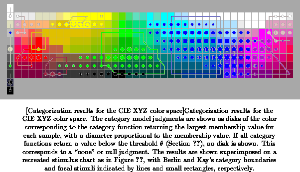
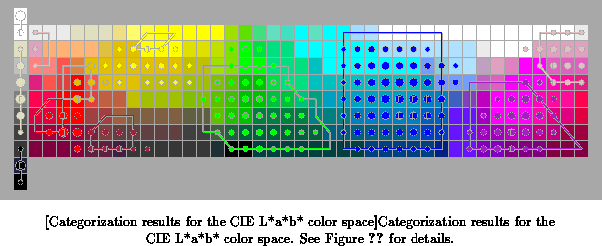
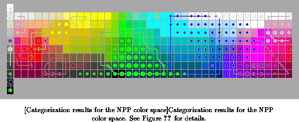
From visual inspection of these figures it is apparent that the
categorization works better in some spaces than in others. In some spaces a
certain category may ``bleed'' outside of the Berlin and Kay category
boundaries, e.g. in the XYZ space, green intrudes into the brown region
(and these two region's boundaries do not touch in the Berlin and Kay
data), and black into green; blue spills over into the purple region,
purple somewhat into pink, white into pink, and green and blue slightly
into gray. Other categories exceed their boundaries without intruding into
another basic category's region, e.g. yellow in all three spaces (but
particularly in L*a*b*). Another type of mismatch is a category that does
not fill enough of its region (which may coincide with exceeding the
boundaries in other areas), e.g. orange, brown, green, blue, and purple in
XYZ. The same type of errors occur in all three spaces, but to varying
extents. The L*a*b* seems to perform best in general, followed by the NPP
space and the XYZ space. Some errors do not seem as serious as others,
e.g. the row of white judgments for the very pale blue and pink stimuli in
the top row in the NPP space does not seem like a particularly serious
mistake, but judging gray as green or blue in the XYZ space or as purple in
the NPP space does. This judgment is qualitative in nature, of course, and
somewhat subjective. In addition, performance on color-related tasks may be
considered more important than this type of theoretical evaluation (see
Chapter ).
To try and get at a more objective measure of performance, we now turn to quantifying the ``goodness of fit'' of the category models. There are two concurrent criteria we can use: how well the extent (area or volume, depending on which representation we use) of a model category fits the extent of the corresponding category in the data, and how close the model focus of each category is to the corresponding category focus (or focal samples) in the data. The following error metric attempts to capture the first of these (the extent of the categories), and is computed over the complete set of Berlin and Kay stimuli
where is the total error (again a Root Mean Square error metric),
is the number of stimuli in the set,
is the predicted (model)
and
is the expected (data) membership value for stimulus
,
is the maximum membership value for stimulus
over all
category model functions,
is the membership threshold as before,
is the category yielding the
,
is the set of all
data categories that the stimulus belongs to (decided by being within the
category boundaries as indicated on Figures
ff.),
is the membership value for stimulus
in model
category
, and
is stimulus
.
The complicated way of determining
is necessary to deal with various cases such as the predicted
category matching or mismatching the expected category, and with discrete
data versus continuous model. In addition to the error over the complete
data set, the square error for each stimulus is added to the running total
for category
iff
i.e. either when the data or the model says it should belong to category
, so we will get an error when the model category is either too small
or too large, as compared to the same category in the data.
The error in the placement of the category model foci is determined as
follows: for each category , determine the stimulus
that is
closest to its focus
, using the regular Euclidean
distance metric on the color space coordinates. This is also the stimulus
with the maximum membership value
, since that is a monotonic
function of distance to the focus. Then the center of gravity
of the data focal stimuli is determined as in
equation
, and finally the focal error is computed as
the Euclidean distance between the two foci:
where is the focal error,
is the number of dimensions of the
color space (in our case 3), and
is the d-th coordinate of point
. This is approximately equivalent to the distance between
the data focus and the orthogonal projection of the model focus onto the
OCS surface (there may be small deviations because the stimuli and data
focus may lie slightly below the OCS surface). The focal error is computed
per category and averaged over all categories.
The computed errors for the color spaces of interest are shown in
Figure to
.
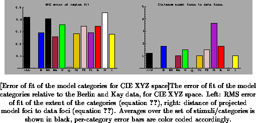
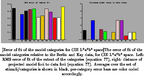
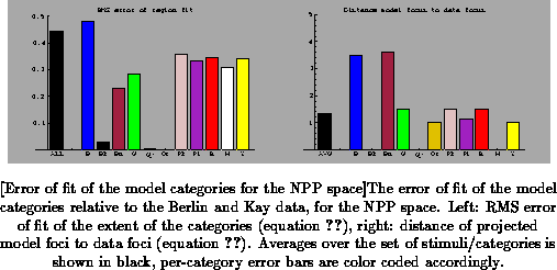
Comparing these figures, we get confirmation that the L*a*b* space performs best in terms of the extent of the color categories (leftmost bar of the left part of the figures, marked ``ALL''). For each of the categories individually except yellow, the error is less in L*a*b* space than in the other two spaces, and for black, gray, and white (i.e. the gray axis), the error is zero in L*a*b* space but not in the other two spaces. Between the RGB and NPP spaces the differences are smaller, with the overall error virtually the same. For some categories such as pink and white the error is smaller in NPP space, for others such as red and yellow the error is smaller in XYZ space. In terms of the error of focus location, the three spaces are comparable overall (leftmost bar marked ``AVG'' in the figures, with some per-category variation among the spaces.